Easier Wall Sensor Calibration

A while back, I posted a way to make simple reflective wall sensor responses appear linear. After struggling with it for a while, it is apparent that it is over complicated. There is an easier way to get acceptable responses…

The previous method is here. While the results are very accurate, the method requires two readings for each sensor to calculate the constants and it is all a bit fiddly to get right. A conversation with Khiew Tzong Yong revealed that he takes only one reading to calibrate his sensors. Have a look again at a typical sensor response with ADC reading plotted against distance from the wall. Here three responses show the effect of walls of slightly different reflectivities.

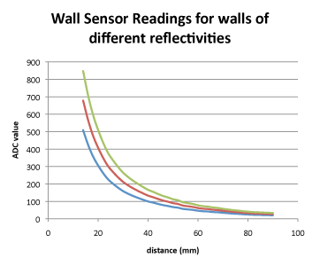
It is not immediately clear from the graphs what is going on although it is easily explained. The red curve represents a ‘standard’ wall. The blue response is from a slightly less reflective wall and the green one from a slightly more reflective wall. Each of these is simply the standard response multiplied by some constant representing wall reflectivity.

As before, these curves are a good fit to an exponential so that we can transform them to a pretty good straight line by taking the logarithm of the ADC reading an calculating 100/ln(ADC). On the mouse, it is convenient to create a table of natural logarithms suitably scaled because it is a relatively expensive operation to calculate them in real time on the mouse. Once transformed, the three responses look like this:

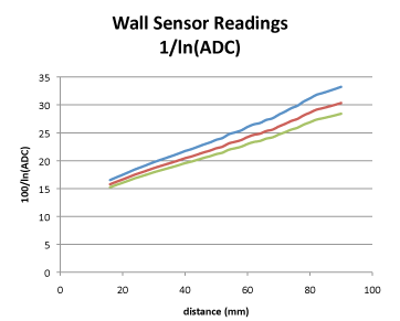
Now the responses look pretty useable for steering but there is still the problem of the wall reflectivity. when the mouse is in the correct position in the maze, the sensor should return a specific value. Suppose I want that to be 100. It doesn’t need to be an actual distance – the important thing is that the value always be in a given range and that, at any actual distance, the response be the same.

All that is needed is to record the actual sensor value at the proper position and use that to scale the responses. So, for this example, I choose the ‘proper’ distance to be 50mm and record the ADC reading at that point (ADC50). All the sensor readings are then converted using the equation Distance = 100*ln(ADC50)/ln(ADC). Clearly, when the sensor is at 50mm from the wall, it must now give a value of 100 once it has been calibrated for that wall. A single reference reading is enough to calibrate the sensor. Now the responses look like this:

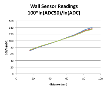
You will see that there is a small change in slope caused by the different reflectivity but otherwise the three responses are now very similar and certainly good enough to use in the mouse.

One caution though. Suppose you callibrate against an odd wall. It soon becomes apparent in contests that not all the walls are as reflective as each other and they may easily vary by 10%. If you are using infra-red sensors, you may not be able to see the difference between lighter and darker walls. The result will be that your mouse may run with an offset – preferring to be a few mm off centre. This will probably not be too much of a problem and you can see mice do this occasionally.

There is some danger in calibrating between two dark walls or between two light walls as that can mess up your steering algorithm depending on how you do it. Always check in a couple of places but the moral is – reflective walls sensors are not highly reliable and should not be relied upon for sub-millimetre accuracy.

Thanks to Khiew Tzong Yong for pointing this method out to me.

Incoming search terms:

• kalman micromouse (1)