Micromouse book
Categories
Recent Comments
Meta
Popular Posts
- Simple ADC use on the STM32 (3,934)
- STM32 Arm-Cortex bootloader (2,657)
- STM32 USART basics (2,534)
- All Japan Micromouse 2011 – finals (1,970)
- STM32F4 – the first taste of speed (1,615)
- Micromouse Book (1,532)
- Nokia 3410 LCD on the STM32 (1,264)
- CodeSourcery GNU Toolchain for the ARM on a Mac (1,097)
- Bit Banding in the STM32 (971)
- ARM STM32 JTAG (921)
Blogroll
-
Upcoming Events
-
Feb6Mon
-
Apr14Sat
-
Tag Archives: sensors
Pointing the sensors
How do you decide where to point the sensors?
I haven’t seen too much discussion on where to point the sensors. The few images I’ve seen show the mouse laterally centered with the diagonal sensors pointed at the pegs for an orthogonal as well as diagonal cell. What is not clear is where the mouse should be longitudinally.
I think the longitudinal location should be a function of the turn radius (and vice versa). The further forward the sensors look, the sooner the mouse can detect the side openings. However, this also means that when it finishes a turn, it may be looking too far forward to do correction or see the pegs.
The other design choice is what should the sensor angle be?
For the sake of this discussion, imagine that a sensor pointed forward (along the longitudinal axis) has an angle of 0 deg. and a sensor pointed directly towards the wall (along the lateral axis) has an angle of 90 deg.
As the sensor angle decreases, the emitter energy reflected by the wall decreases which means that the detector response goes does. Also, as the sensor angle decreases, a change in the mouse angle has a larger effect on the detector’s response.
So, my design target has been to put the mouse in the middle of a cell and then locate the sensors such that they can see the longitudinal peg and maximize the angle of the sensor. Since nothing is for free, as you maximize the angle of the sensor, you have to move it further away from the center of the mouse which means you are increasing the sensor’s rotational inertia contribution.
For the longest time, I wondered why people were crossing the diagonal sensors i.e. the sensor on the left side of the mouse looked at the right wall and vice versa? The answer turns out to be that they were trying to minimize the rotational inertia! Since light drops off at 1/distance^2 (Peter has some graphs in one of his blog posts), this means they were trading off sensor performance also.
As they say, mouse design is full of compromises.
You might want to move paper cut outs of the mouse along with pieces of paper showing the sensor location and angle through a maze to get an idea of different sensor angles. Alternatively, you might be able to do this with a CAD program – my CAD skills are too limited for me to have tried this.
Decimus 2 sensor geometry
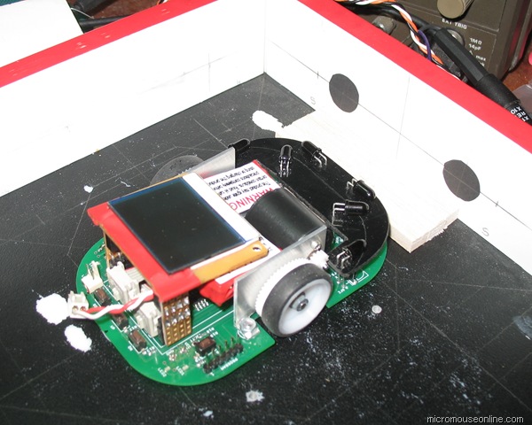
Decimus 2 is now nearly ready to go. I don’t have much hope of having it ready for the Japan contest but it is worth a try. The mouse weighs only 2/3 as much as its predecessor at about 115g with batteries. This weight saving is almost entirely due to the use of the new 1717 size motors. It looks like everything is working so today, I set up the sensors. These have a different alignment to those I have used before.
The forward sensors now point outwards a little. This should give two benefits. First, they will be more sensitive to the presence of walls and posts when running diagonals. Second, there are some possible issues with the shininess of maze walls. By trying to avoid having any sensor pointing at 90 degrees to a wall, the effect of that shininess should be mitigated to a certain extent. Since the forward-facing sensors are quite important for adjusting forward errors and alignment, they need to be reliable. This is a relatively new requirement for my mice as I find new uses for the forward sensors.
The side sensors are nor angled forwards a little for a similar reason. Also, since these have been the primary sensors used for wall edge detection, they now do that a bit further in advance without giving up too much accuracy if the mouse is not well aligned.
The diagonal sensors point slightly more to the rear than before. I hope his will make them a little more reliable for steering as it will place the response further in the shallow part of the curve when there is a rotational error. They can now also be used more reliably for edge detection. The downside is that they will give an edge later than before which may make it harder to do the diagonal turns.
The edge detection is quite critical to the execution of a good turn. If you can get a reliable edge – which must always exist before a turn – then you can use that to initiate the turn.
Aligning the sensors is made much easier by use of my trusty Sony video camera. Althoug not the latest and greatest model it has one major advantage. the Super-nightshot mode allows you to move the IR filter out of the way and view the IR produced by the sensors. Aligning the emitters to appropriate marks on the walls is pretty easy then. After they are aligned, each is held in place with a little epoxy glue. I use the slow setting, standard type as it flows a little to make a nice support for the emitter. you need to be absolutely sure of your setup before applying the epoxy though. Once done, there is not much opportunity for undoing it.
Line Follower Sensors Setup
With the sensors installed and the robot pretty well complete, it is time to see if they can actually do the job they were designed for. the idea is that the line of sensors will be able to measure the robots offset from the centre of the line over as wide a range as possible.
In a previous post, I described how the error could be determined very conveniently by looking at the difference in reading between two sensors. This is very true and perfectly valid for the case where there are three sensors. Or even two. However, I put five on Bob and wanted to get as much of a displacement as possible. After messing with the simple difference technique for a bit I decided to get on and do the job ‘properly’. Well, as properly as I could think of today at any rate.
Bob has five sensors arranged at fixed intervals of 0.5 inch. This spacing is determined mostly by the fact that the sensors are mounted on 0.1" pitch perfboard. The fixed spacing turns out to be important and very convenient. A typical set of sensor readings look like this:
| Sensor | 0 | 1 | 2 | 3 | 4 |
| Reading | 127 | 124 | 9 | 45 | 125 |
the sensors are numbered from left to right from the driver’s point of view. Each reading has been normalised to a maximum value of 127 representing the black background so the low values are sensors that can ‘see’ the white line. It should be apparent that the robot is off centre to the left by some small amount as sensor 3 can see the line but not as well as sensor 2. Usually only two sensors can see the line at once. The spacing is such that, as soon as sensor three stops seeing the line, sensor 1 starts to see it. A slightly closer spacing would be better for the technique I am describing. I think a sensor spacing equal to the line width would be best.
So, we are interested in the response of three sensors. The one with the lowest reading and the sensor either side of that. We can plot the readings on a graph and try to fit a curve to the three we are interested in. Something like this:
The curve is a quadratic and you can see that the turning point – the minimum value – is in between sensors 2 and 3. It is closer to sensor 2 as you might expect. Without drawing lots of examples, it should also be apparent that the turning point will move toward sensor 3 as the reading on that sensor gets smaller and that on sensor 2 gets bigger. In fact, that turning point allows us to interpolate the actual centre of the line quite accurately as long as the sensor spacing is regular and appropriate. On BOB they are a bit far apart but it still works out quite well.
How can we find the turning point? the curve is a quadratic and we have three points that lie on it. thus the equation can be solved using simultaneous equations. Remember those? A technique for solving these things is to calculate differences. Again, I won’t detail the entire process but just give the result.
We have three sensor readings s1, s2 and s3 corresponding to the position of three sensors at positions x1, x2, x3. If we take the distance between the sensors to be a single unit, the position of the turning point, relative to s2 is:

Only the division need cause any problems for the code and I am using C so I can let the compiler deal with that. To help with the division and to ensure there are no overflows or underflows, it is convenient to perform the first part and then pre-scale it by 256 before doing the division. The result will be a number between -128 and +128 representing the offset of the turning point from the middle of the three sensor readings.
To test out the theory on Bob, I made up a rough test rig which would allow me to move a white line under the sensors in increments of 5mm and have the robot calculate its offset from centre. The test rig picture is at the top of this page. Here are a typical set of results:
Not perfect but they seem to do the job. The offset can be calculated over the full range of +/- 25mm from the centre. The results seem monotonic and fit a straight line quite well. Better spacing should improve this a bit but I shall leave them as they are for now. The way the ends of the range are dealt with could be improved since it should be possible to get good results out as far as +/- 40mm with this technique. Time is short however, so I will go with this for now
Line follower sensor experiments
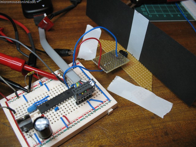
The simplest arrangement for a line follower is probably two sensors with digital outputs. As long as one can see the line and the other can see the background, the controller is happy otherwise it must turn left or right as appropriate. I was after something a bit more sophisticated for Bob the Line follower…
The first task it to examine the behaviour of a single sensor. To this end, a version of the Bob controller was made up on a breadboard and a single TCRT5000 sensor attached to a remote board. Black card has a white stripe added in the same way as the track. That is a single layer of cheap, 19mm white PVC tape. With the card mounted vertically, the sensor can be placed at varying distanced from the vertical track. A piece of perfboard taped to the desk lets me measure the distance between the sensor and the track as well as the lateral displacement. In this way a series of measurements can be taken as the sensor is moved across the track at different distances. All the room lighting is fluorescent with negligible IR content. The emitter is supplied from 5V through a 220 Ohm current limiting resistor. The phototransistor has a 10 kOhm resistor to the collector and thence to the 5V supply. Voltage are measured at the collector. The result of several trials is shown below:

Dimensions are in inches. The results are entirely predictable. With the sensor close to the track, the edges are more clearly defined and the contrast between on-track and off-track are greatest. Readings across the width of the track are fairly equally matched. Such a response would be ideal for a sensor connected to a schmidt trigger input on a processor and would be likely to give reliable, clean indications of when the sensor was over the track.
As the sensor is moved further away, the response to the track is smaller and the edges less distinct. By the time it gets to be 0.4 inches away, it seems likely that there would not be a large enough response to trigger a processor digital input. Although not shown, very small distances can be quite problematic as these sensors have a tab that prevents the detector from directly seeing the emitter. When that is in contact with the track, although the reflected light is very strong, the tab prevents the detector seeing it.
The really interesting area is between about 0.3 and 0.4 inches above the track. Here we still get a fairly strong response but the reading varies continuously as the track passes in front of the sensor. this is particularly useful as it tells us not just where the edge of the track it but give an indication of how far away from it we are and leads to the possibility of measuring displacement quite accurately. Having only a single sensor, I replicated the results for a distance of 0.3 inches and arranged them in three sets in a spreadsheet to simulate three sensors space 0.5in apart. These results can then be combined in a single graph:

At that spacing, you can see that the responses overlap slightly. As the track moves away from the central position with the no.2 sensor directly over it, the adjacent sensor responses grow. the purple line is the difference between the left and right sensors and this result looks particularly promising. It is always positive when we are in error one way and always negative when we are in error the other way. When we are positioned most accurately over the line, the slope of the error is greatest making the controller most sensitive to error. All in all, fro displacements up to about +/- 0.6 inches, this looks like an ideal error function allowing us to calculate offset to a fine degree. The addition of another two sensors outside these three will extend the range of errors to at least +/- 1 inch. As the robot strays outside the error range indicated in the graph above a different pair of sensors can be used for the correction. It could be as simple as using the sensor either side of the one that is giving the largest reading. With care taken over what happens when only the outermost sensors can see the line, this should give a robust and accurate error function over a wide range of errors. Experiments with the actual sensor array will test this assertion. Or, at least, they will if I can get the serial comms working on Bob…
New line follower robot
Line followers are a perennial favourite of the small robot builder. It is not hard to make something that will bumble about and follow a line marked out on the floor. the technology can be very simple but the same basic idea is used in sophisticated robots on factory floors. The tricky part is in making the line-follower fast and smooth in its response. Whether or not I can do that remains to be seen but I am going to have a go …
There has been a bit of discussion lately about a simple line-following competition to replace a couple of the schools contests at the micromouse events. You can see the proposal on the forum:
http://www.micromouseonline.com/forum/viewtopic.php?f=3&t=281
So that there is at least one entry, I agreed to build a follower in time for the November RoboTic event in Birmingham (http://www.tic.ac.uk/micromouse/ROBOtic08.asp).
Right, the question is, what to make it out of. I looked at various options for motors and was about to order some small gearmotors. These came in at about £12 each and would need wheels making and tyres fitting.
For the controller, I chose aPIC18F252 because I happened to have three of them spare. the newer 18F2520 might be a better choice now. the PIC is handy because development tools in the form of MPLAB, the PicKit2 and a C compiler are easy to get. The software is free and the PicKit2 can be had for very little cost considering its versatility.
Sensors are the Vishay TCRT5000 IR reflective sensor available from Farnell among others. With an eye to future development, I chose to put five sensors in the beast. This should give me better than needed resolution and will allow a ‘proper’ PD controller rather than the usual on-off type of control seen when only using two detectors. Of course, various simpler digital control schemes can be tried anyway with these sensors. I was specifically looking for versatility so that I can experiment with a range of strategies.
To drive the motors, I was going to use the ubiquitous L293D. However, these are not terribly cheap now and I have no obvious requirement to drive the motors in any direction other than forwards. After a poke about in the parts trays, I found a collection of TIP122 Darlington transistors. These will handle plenty of current. To be on the safe side, I added flyback diodes across the motors although I would expect the TIP122 to survive anything these little motors can generate. We will soon see.
With all the parts decided, it is time to get building.
Sensor alignment
For consistent results, the sensors on a micromouse need to be carefully aligned and then fixed in place. In a perfect world, the emitters would all have the same radiation pattern and would generate the same amount of illumination for a given current. Well, that is never going to happen without hand-picking the devices. That would take a long time so we make do with what we have and work around their limitations. Similarly, the detectors have variations to cope with as well. The first step is to get the emitters lined up and pointing where they should…
A small section maze – well, one square, is set up on the bench for the alignment process. Simple jigs and lines drawn on the floor allow the mouse to be positioned exactly and repeatably in relation to the walls. On the walls a series of pencil marks show where the emitters should have their beams pointing. To detect the IR beams, I have a cheap webcam modified to allow it to respond to IR light. This is an easy adaptation in many webcams and just involved removing a filter and replacing it with a material opaque to visible light but transparent to IR. If you still have some old floppy disks handy, the recording film on those is good for that.
The converted camera is actually too sensitive and produces very poor pictures so a bit of fiddling is needed to get good results. A much better alternative would be a handy-cam like some of the Sony types that can be set to respond to IR.
To help see where the IR is falling, small circles of black paper are placed over the points where the beam should lie. These reflect much less light than the walls and makes it much easier to see with the now over-sensitive camera. To an extent, you can also use the black disks by aligning the emitters so that a minimum of light is reflected to the detectors. If the disks are the right size for the emitter pattern this can be quite reliable but the camera is better.
Once the emitters have been lined up, they are fixed in place with epoxy glue. You really need to get this right. Changing things later is not an easy option. Try not to burn out an emitter!. The emitters on Decimus are well shielded from the detectors. Even so, it is a good idea to put a short length of heatshrink tubing around them as that will make it a bit easier to replace them later if necessary.
With the emitters aligned, the detectors can be moved about to give a reasonable range of results. The sensors are arranged in pairs but it is very unlikely they will give closely similar responses so some software compensation will be needed. This can be simple threshold values or complete look-up tables. Don’t however get to tied in to the values that work for your particular maze walls. Remember that the mouse will have to work in any maze under a variety of lighting conditions.
Feeling our way with sensors
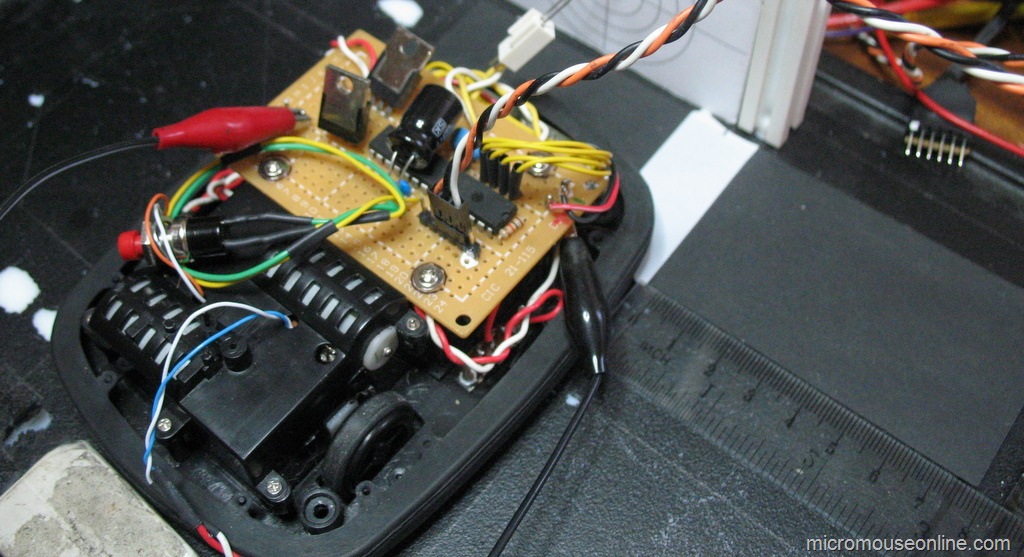
The sensors are a critical part of a micromouse. Primus uses six infra-red reflective sensors. Here is code to test that they are working.Now that we have a nice display to show what the sensor reading are, we can get that module tested. Since the hardware is very simple, there is not a lot to go wrong. Yet somehow I had a dead sensor when I first tested the Primus prototype. It was a simple dry joint that would have been detected by more careful inspection of the board.This program just sets up the sensor hardware and activates each channel in turn. All six channels are then displayed on the screen as raw ADC values. there is no real need to scale these numbers. If it is working correctly, each channel should show values between nearly zero and about 700 or so.For best performance the sensors will need careful alignment. For now, just check that they are working. They should easily detect the presence of a wall at distances of 150mm and should not saturate until the wall is only about 35-40mm away.The reason the maximum value is only about 700 is that the TSL262 can only reach a maximum output value of around 3.5V. You should find that the sensors are relatively immune to ambient light levels although they will become less sensitive under very bright conditions. A black paper or card shield is needed over the TSL262s to reduce the effect of ambient light.The sensor module is also responsible for measuring battery voltage via a potential divider on the battery input. While not essential for use with NiMh or NiCd cells, it is particularly important that LiPo cells do not become discharged to too low a level. You program can monitor the battery voltage and sound an alarm or shut the mouse down if the battery voltage gets too low. The processor will carry on as long as the voltage into the regulator does not drop below about 7V so you should have plenty of time to avoid trouble.The project files can be downloaded here:primus4.zip Continue reading
Sensor Data Analysis
Micromouse sensors are subject to several sources of error and interference. Capturing a set of data samples lets you do some simple analysis of the effects of those errors.The test rig was set up with a section of wall placed at about 50mm from the sensors. This gives a large reading where noise and interference should be a small proportion of the results. 4096 samples were taken at approximately 250Hz and the results analysed in Excel with the built-in data analysis tools. First we have the raw data:
Here you can see that noise accounts for about 1-2% of the sensor reading. This is perfectly acceptable in this application and should cause no problems for the mouse. Probably half that would be quantisation noise from the ADC converter. The larger spikes are probably side effects of not having taken the trouble to write a ‘proper’ test program so there are several interrupt sources upsetting the timing. The spikes show, I think, periodic beating between the sample rate and the background interrupts. I should really eliminate that effect but…Next the results are arranged into a histogram. If the noise were purely random (Gaussian), you might expect a nice bell-shaped curve.
Well, that seems a bit odd at first sight. However, for this test I had arranged that there would be some incandescent lighting. As this is not very bright in the room where the tests were done, I placed the bench magnified over the test setup to concentrate the light from the overhead lamp onto the test area. With sinusoidal interference overlaid on the data, this is exacly the kind of result you might expect. The actual sensor reading is somewhere in between the peaks which are the result of the interference.Processing the data with a Fast Fourier Transform (FFT) should show up any periodic interference in the results.
Sure enough, there is a distinct peak at about 100Hz – exactly where you would expect it where there is incandescent ambient lighting in the UK. A quick check of the statistical analysis gives a standard deviation of about 2.8These tests were repeated with the wall at about 120mm from the sensor where the average sensor reading was around 100. Here the interference would be a larger portion of the result. Once again the standard deviation is about 2.5 but this now represents an error five times greater than before. You would, of course expect signal to noise ratio to worsen as the distance increases. Even so, maximum expected errors are still quite acceptable over the normal working range of the sensor. These sensors are normally used for steering over a quite restricted range of distances around 80mm or so. Continue reading
Sensor test
The simple sensor circuit described by Ng Beng Kiat seems to give the best results.On his web site (http://www.np.edu.sg/alpha/nbk/) Beng Kiat describes Min4, one of his recent mice. In there is a PDF with schematics for the mouse. The sensor circuit for Primus is essentially the same except for a couple of component value changes. The emitters are run in series pairs from the 5V supply. Not shown here, a ULN2003 darlington driver does the switching.
The TSL262 is used as a detector. Although Beng Kiat’s circuit shows a Shottky diode, it is omitted from this version as tests indicate they serve no apparent purpose in this design. Another change is to the values of the AC coupling components. This has little discernable effect on the circuit operation but 33nf ceramic capacitors in a suitable size are relatively hard to come by whereas 100nF items are cheap and plentiful as they are used universally for power supply decoupling.
A simple test rig for this circuit allowed me to generate a graph of analogue reading against distance. The ADC is operating in 10 bit mode so full scale is 1023. Note that the TSL262 cannot bring its output above about 3.75V. although the data sheet indicates that this can be extended with a resistor from the output to Vdd, it seems to have little effect in this circuit.
While very non-linear, beyond abut 30mm, the results are completely monotonic. That is, as distance increases, reading always decreases. Closer than 30mm, the physical arrangement of the sensor assembly prevents the sensor from seeing the spot of light. It is not a good idea to compensate too much for this as we can arrange that the sensors are only used at distances greater than 40mm from a wall. Notice that it is quite easy to detet the presence of a wall at distances of at least 120mm. there is not, however, enough of a response to be sure of seeing a wall in an adjacent cell. Continue reading


Add to Google